Laminar pipe flow calculations for non-Newtonian fluids
[1]:
import numpy as np
import matplotlib.pyplot as plt
%matplotlib inline
import rheoflow
Nomenclature
This notebook provides deep examples for using rheopy for pipe flow. Both tube and slit flow examples with a variety of viscosity models are provided. SI units units are used everywhere. For the variables used here, the units are:
\(\eta = \left< Pas \right>\)
\(\sigma = \left< Pa \right>\)
\(\dot{\gamma} = \left< s^{-1} \right>\)
\(\Delta P = \left< Pa \right>\)
\(Q = \left< \frac{m^3}{s} \right>\)
\(v_z = \left< \frac{m}{s} \right>\)
\(length = \left< m \right>\)
\(radius = \left< m \right>\)
Calculation procedure
The rheopy.laminar notebook is intended to work with any viscosity model. There are four elemenets of computation:
- A viscosity model using the class structure provided - \(\eta(\dot{\gamma})\)
- Shear rate calculation at any radial position (tube) or height (slit) - \(\dot{\gamma}(r)\)
- Velocity calculation at any position - \(v_z(r)\)
- Volumetric flow rate - \(Q\), given \(\Delta P\) (or vice versa)
Details of calculations
1 - Viscosity model
Use pre-existing, or create new function with viscosity as a function of shear rate:
\(\eta \left[ \dot{\gamma} \right]\)
2 - Shear rate calculation (\(\dot{\gamma}\))
The equation to be solved for shear rate at any radial position is
\(\eta \left[ \dot{\gamma}(r) \right] \dot{\gamma}(r) = \frac{r}{2} \frac{\Delta P}{L}\),
where \(\dot{\gamma}(r) = \frac{d v_z(r)}{dr}\)
This equation is simply an equality of shear stress from constituitve model and shear stress from a momentum balance. This calculation is numerical in rheopy because this equation does not always have analytical solutions. The Carreau viscosity model is an example where an analytical solution does not yet exist.
Note that 4 inputs are required: 1. Viscosity model - \(\eta(\dot{\gamma})\) 2. Tube radius 3. Tube length 4. Pressure drop (\(\Delta P\))
3 - Velocity calculation (\(v_z\))
The axial velocity is calculated from the shear rate directly
\(v_z(r) = -\int_{r}^{R} \dot{\gamma}(r)dr\)
This integral is computed numerically beacuse the shear rate is computed numerically.
4 - Volumetric flow rate (\(Q\))
The volumetric flow rate is computed by numerically integrating the velocity profile
\(Q = 2\pi \int_{0}^{R} v_z(r)rdr\)
Note that if Q is an input, then \(\Delta P\) must be solved for iteratively.
Viscosity model class structure
The actual class of power_law is shown below. Any viscosity model class must have three features: 1. A init method to initialize an object 2. A str method to print the object (not actually required) 3. A calc_visc method for computing the viscosity for input shear rate
[2]:
class power_law(rheoflow.viscosity.property_plot):
    def __init__(self,name='Default',k=1.,n=.5):
        self.name = name
        self.k = k
        self.n = n

    def __str__(self):
        return str(self.name+'\n'+
            'k ='+str(self.k)+'\n'+
            'n='+str(self.n)+'\n')

    def calc_visc(self,rate):
        return self.k*(rate+1.e-9)**(self.n-1.)
An instance, pl_viscosity, of the power_law class is created. The object is printed, showing parameter values. The viscosity at a shear rate of 150 \(s^{-1}\) is computed.
[3]:
pl_viscosity = power_law(name='My example power-law',k=2.0,n=0.7)
[4]:
print(pl_viscosity)
My example power-law
k =2.0
n=0.7
[5]:
pl_viscosity.calc_visc(rate=150.)
[5]:
0.4448387563894917
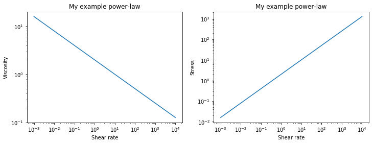
The inherited laminar.property_plot provides convenience methods. For example viscosity_plot and stress_plot are ised here. The min and max shear rate range in the plot are .001 and 10,000.
[6]:
pl_viscosity.visc_plot()

[7]:
plt.figure(figsize=(12,4))
plt.subplot(121)
pl_viscosity.visc_plot()
plt.subplot(122)
pl_viscosity.stress_plot()
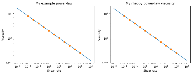
We can instantiate an object, rheopy_pl_viscosity, from rheopy.laminar that is the same. It produces the same results.
[8]:
rheoflow_pl_viscosity = rheoflow.viscosity.power_law(name='My rheopy power-law viscosity',k=2.0,n=0.7)
[9]:
plt.figure(figsize=(12,4))

rate_list = np.logspace(-2,3,11)
visc_list = [pl_viscosity.calc_visc(rate=r) for r in rate_list]

plt.subplot(121)
pl_viscosity.visc_plot()
plt.plot(rate_list,visc_list,'o')
plt.subplot(122)
rheoflow_pl_viscosity.visc_plot()
plt.plot(rate_list,visc_list,'o')
[9]:
[<matplotlib.lines.Line2D at 0x151c703f28>]
Laminar pipe class structure
An instance of the class laminar_tube_flow is created. The instance/object is called my_tube. The object is created using the viscosity model pl_viscosity that we used above.
[10]:
my_tube = rheoflow.pipe.laminar(name='My experimental tube',radius=.005,length=5.,viscosity=pl_viscosity)
The object my_tube may be printed to see important variables. Note that neither pressure drop or flow rate have been specified so nothing is computed.
[11]:
print(my_tube)
Name =My experimental tube
Radius =0.005
Length =5.0
Pressure drop =None
Flow rate =None
Shear rate wall = None
Now we set a value of pressure drop tp 50,000 Pa. Then when we print my_tube, a flow rate and shear rate are computed.
[12]:
my_tube.pressure_drop = 500000.
[13]:
print(my_tube)
Name =My experimental tube
Radius =0.005
Length =5.0
Pressure drop =500000.0
Flow rate =8.777724882195872e-05
Shear rate wall = 989.887255479541
The variables (attributes) of my_tube may be accessed. They are the same values as seen in the print statement.
[14]:
my_tube.q
[14]:
8.777724882195872e-05
[15]:
my_tube.pressure_drop
[15]:
500000.0
[16]:
my_tube.shear_rate_wall
[16]:
989.887255479541
[17]:
my_tube.shear_stress_wall
[17]:
250.0
[18]:
my_tube.radius
[18]:
0.005
Now we can change a variable, such as radius, and observe the new calculated values of my_tube.
[19]:
my_tube.radius = .01
[20]:
print(my_tube)
Name =My experimental tube
Radius =0.01
Length =5.0
Pressure drop =500000.0
Flow rate =0.001890230657570641
Shear rate wall = 2664.5788956677325
[21]:
my_tube.radius = .005
my_tube.length = 2.0
[22]:
print(my_tube)
Name =My experimental tube
Radius =0.005
Length =2.0
Pressure drop =500000.0
Flow rate =0.00032498827405481125
Shear rate wall = 3664.9787386218486
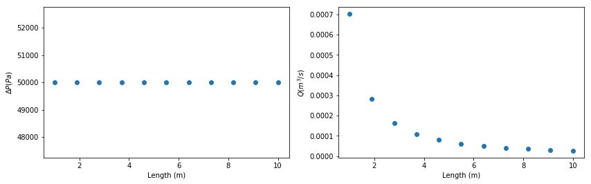
Change length example
We can also create lists of variables, such as tube length. Then we can explore and plot in a pythonic way. Here we create a list, length_list, with values from 1-10 m. Then we plot the resulting changes.
Note that pressure drop does not change unless we explicitly change the flow rate to a new value. So pressure drop does not change in the first plot. However, flow rate changes with length in the second plot.
[23]:
length_list = np.linspace(1.,10.,11)
my_tube.q = 1.e-6
my_tube.pressure_drop = 50000.
my_tube.radius = .01

dp_list = [my_tube.pressure_drop for my_tube.length in length_list]
q_list = [my_tube.q for my_tube.length in length_list]

plt.figure(figsize=(14,4))
plt.subplot(121)
plt.plot(length_list,dp_list,'o')
plt.xlabel('Length (m)')
plt.ylabel('$\Delta P (Pa)$');
plt.subplot(122)
plt.plot(length_list,q_list,'o')
plt.xlabel('Length (m)')
plt.ylabel('$Q (m^3/s)$');
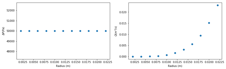
Change radius example
We can also create lists of variables, such as tube radius. Then we can explore and plot in a pythonic way. Here we create a list, radius_list, with values from .002-0.22 m. Then we plot the resulting changes.
Note that pressure drop does not change unless we explicitly change the flow rate to a new value. So pressure drop does not change in the first plot. However, flow rate changes with radius in the second plot.
[24]:
radius_list = np.linspace(.002,.022,11)
my_tube.q = 1.e-6
my_tube.pressure_drop = 50000.
my_tube.length = 1.
dp_list = [my_tube.pressure_drop for my_tube.radius in radius_list]
q_list = [my_tube.q for my_tube.radius in radius_list]

plt.figure(figsize=(14,4))
plt.subplot(121)
plt.plot(radius_list,dp_list,'o')
plt.xlabel('Radius (m)')
plt.ylabel('$\Delta P (Pa)$');
plt.subplot(122)
plt.plot(radius_list,q_list,'o')
plt.xlabel('Radius (m)')
plt.ylabel('$Q (m^3/s)$');
Carreau viscosity model pipe flow example
Carreau viscosity model
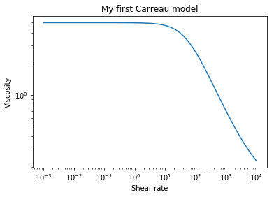
The Carreau viscosity model may be expressed with four parameters as:
\(\eta \left( \dot{\gamma} \right) = \eta_{\infty}+ \frac{\eta_0-\eta_{\infty}}{\left( \left( 1+\left(\lambda \dot{\gamma} \right)^a \right) \right)^{\frac{1-n}{n}}}\)
To instantiate an object of class Carreau, we use
[25]:
my_carreau_model = rheoflow.viscosity.carreau('My first Carreau model',
                                   eta0=5.,etainf=.11,reltime=.02,a=1.3,n=.3)
[26]:
my_carreau_model.calc_visc(rate=10.)
[26]:
4.7030017198606435
[27]:
print(my_carreau_model)
My first Carreau model
eta0 =5.0
etainf =0.11
reltime =0.02
a =1.3
n=0.3
[28]:
my_carreau_model.visc_plot()
Laminar pipe flow with Carreau viscosity model
[29]:
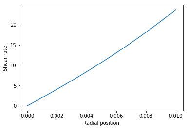
my_carreau_tube = rheoflow.pipe.laminar('my laminar flow pipe',density=1000.,
                               radius=.01,length=1.0,viscosity=my_carreau_model)
[30]:
my_carreau_tube.pressure_drop = 20000.
[31]:
print(my_carreau_tube)
Name =my laminar flow pipe
Radius =0.01
Length =1.0
Pressure drop =20000.0
Flow rate =1.782691971171862e-05
Shear rate wall = 23.673966897448867
[32]:
my_carreau_tube.shear_rate_wall
[32]:
23.673966897448867
[33]:
my_carreau_tube.shear_stress_wall
[33]:
100.0
[34]:
my_carreau_tube.shear_rate_plot()
[35]:
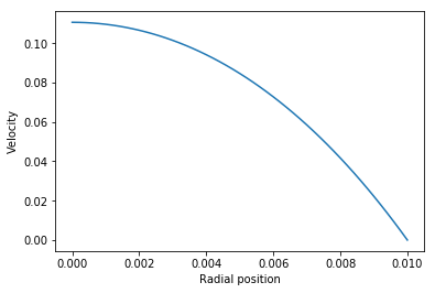
my_carreau_tube.vz_plot()
[36]:
my_carreau_tube.pressure_drop
[36]:
20000.0
[37]:
my_carreau_tube.q
[37]:
1.782691971171862e-05
[38]:
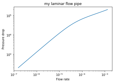
my_carreau_tube.q_plot(pressure_drop_min=200.,pressure_drop_max=200000.)
Three component model pipe flow example
Three component viscosity model
The 3-component viscosity model may be expressed with three parameters as:
\(\eta \left( \dot{\gamma} \right) = \frac{\tau_y}{\dot{\gamma}} + \frac{\tau_y}{\dot{\gamma}}\left( \frac{\dot{\gamma}_{crit}}{\dot{\gamma}}\right)^n + \eta_{bg}\)
To instantiate an object of class Three_component, we use
[39]:
my_3c_viscosity = rheoflow.viscosity.three_component('my 3-comp viscosity model',tauy=100., \
                            gamma_crit=10., eta_bg=1.,m=1000.)
[40]:
plt.figure(figsize=(10,8))
plt.subplot(221)
my_3c_viscosity.visc_plot()
plt.subplot(222)
my_3c_viscosity.stress_plot()

Laminar pipe flow with three-component viscosity model
[41]:
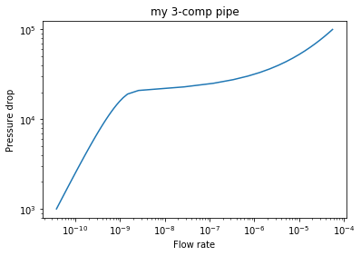
my_3c_pipe = rheoflow.pipe.laminar('my 3-comp pipe',density=1000.,
                radius=.01,length=1.,viscosity=my_3c_viscosity)
[42]:
my_3c_pipe.pressure_drop = 200000.
[43]:
print(my_3c_pipe)
Name =my 3-comp pipe
Radius =0.01
Length =1.0
Pressure drop =200000.0
Flow rate =0.00021750103142115598
Shear rate wall = 327.61947052473454
[44]:
my_3c_pipe.q_plot(pressure_drop_min=1000.,pressure_drop_max=100000.)
[45]:
my_3c_pipe.pressure_drop=50000.
my_3c_pipe.q
[45]:
8.4884073546493e-06
[46]:
my_3c_pipe.q = 8.4884e-6
my_3c_pipe.pressure_drop
[46]:
49999.98759870919
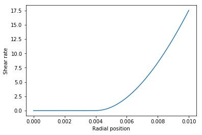
[47]:
my_3c_pipe.shear_rate_plot()
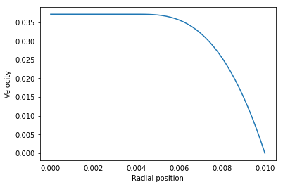
[48]:
my_3c_pipe.vz_plot()
[ ]: