Quickstart for non-Newtonian pipe flow calculations¶

All units are SI.

Nomenclature¶

This notebook provides deep examples for using rheopy for pipe flow. Both tube and slit flow examples with a variety of viscosity models are provided. SI units units are used everywhere. For the variables used here, the units are:

\(\eta = \left< Pas \right>\)

\(\sigma = \left< Pa \right>\)

\(\dot{\gamma} = \left< s^{-1} \right>\)

\(\Delta P = \left< Pa \right>\)

\(Q = \left< \frac{m^3}{s} \right>\)

\(v_z = \left< \frac{m}{s} \right>\)

\(length = \left< m \right>\)

\(radius = \left< m \right>\)

[1]:

import numpy as np
import matplotlib.pyplot as plt
%matplotlib inline
from ipywidgets import interact, interactive, fixed, interact_manual
import ipywidgets as widgets
from IPython.display import display, Math, Latex
import rheoflow

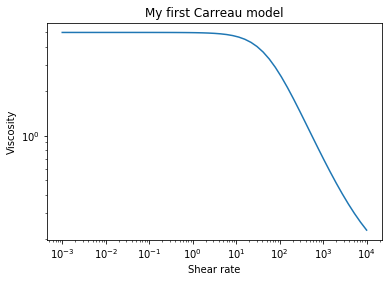
Step 1 - Specify a viscosity model¶

The variable (object) name is up to the user. Here we use my_carreau_model as the name for a Carreau viscosity model with associated parameters.

The details of rheoflow.viscosity.carreau may be viewed by typing help(rheoflow.viscosity.carreau). A list of all viscosity models currently implemented may be accessed by typing help(rheoflow.viscosity).

The python code is all viewable in viscosity.py

[2]:

my_carreau_model = rheoflow.viscosity.carreau('My first Carreau model',
                    eta0=5.,etainf=.11,reltime=.02,a=1.3,n=.3)

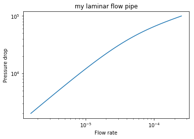
Step 2 - Specify a pipe using the viscosity model¶

The variable (object) name is up to the user. Here we use my_carreau_tube as the name for a laminar pipe flow object with associated parameters. The viscosity model defined (instantiated) above is used.

The pipe has the following attributes:

radius = 0.01 m, length = 1.0 m, fluid density = 1000 kg/m^3

[3]:

my_carreau_tube = rheoflow.pipe.laminar('my laminar flow pipe',density=1000.,
                               radius=.01,length=1.0,viscosity=my_carreau_model)

Step 3 - use the pipe flow object¶

Initially, neither pressure drop or flow rate were specified.

[4]:

print(my_carreau_tube)

Name =my laminar flow pipe
Radius =0.01
Length =1.0
Pressure drop =None
Flow rate =None
Shear rate wall = None

Specifiy a pressure drop

[5]:

my_carreau_tube.pressure_drop = 20000.

[6]:

print(my_carreau_tube)

Name =my laminar flow pipe
Radius =0.01
Length =1.0
Pressure drop =20000.0
Flow rate =1.782691971171862e-05
Shear rate wall = 23.673966897448867

Accessing attributes of a pipe object¶

[7]:

my_carreau_tube.q

[7]:

1.782691971171862e-05

[8]:

my_carreau_tube.pressure_drop

[8]:

20000.0

[9]:

my_carreau_tube.radius

[9]:

0.01

[11]:

my_carreau_tube.shear_rate_wall

[11]:

23.673966897448867

[12]:

my_carreau_tube.shear_stress_wall

[12]:

100.0

Modifying attributes of a pipe object¶

[13]:

my_carreau_tube.q = .0001

[14]:

print(my_carreau_tube)

Name =my laminar flow pipe
Radius =0.01
Length =1.0
Pressure drop =65281.39307599825
Flow rate =0.0001
Shear rate wall = 157.32118720688686

[15]:

my_carreau_tube.pressure_drop = 40000.

[16]:

print(my_carreau_tube)

Name =my laminar flow pipe
Radius =0.01
Length =1.0
Pressure drop =40000.0
Flow rate =4.376689029902029e-05
Shear rate wall = 62.29932871052237

A few convenience plots¶

[18]:

my_carreau_model.visc_plot()

[20]:

my_carreau_tube.q_plot(pressure_drop_min=2000.,pressure_drop_max=100000.)

[21]:

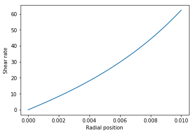
my_carreau_tube.shear_rate_plot()

[22]:

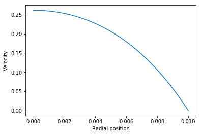
my_carreau_tube.vz_plot()

[ ]: